데이터 소개

- PFCN dataset사용
- 원본의 경우 800*600의 사람 이미지와 배경에 대한 흑백 이미지
- 작은 용량의 pfcn_small데이터 사용
- 데이터 출처 : pfcn_original, pfcn_small
데이터 불러오기
import tensorflow as tf
from tensorflow import keras
from keras.layers import Dense
from keras.models import Sequential

import pandas as pd
import numpy as np
import matplotlib.pyplot as plt
import seaborn as sns
import warnings
from IPython.display import Image

warnings.filterwarnings('ignore')
%matplotlib inline

SEED = 34

#colab연동
from google.colab import drive
drive.mount('/gdrive', force_remount=True)
!ls -al /gdrive/'My Drive'/'Colab Notebooks'/data/pfcn_small.npz

pfcn_small = np.load('/gdrive/My Drive/Colab Notebooks/data/pfcn_small.npz')
train_images = pfcn_small['train_images']
train_mattes = pfcn_small['train_mattes']
test_images = pfcn_small['test_images']
test_mattes = pfcn_small['test_mattes']

print(train_images.shape)
print(train_mattes.shape)
print(test_images.shape)
print(test_mattes.shape)
train_images.dtype
float64 타입의 1700개 train데이터와 300개의 test데이터로 구성.
- 데이터 확인
plt.imshow(train_images[0])
plt.show()
plt.imshow(train_mattes[0])
plt.show()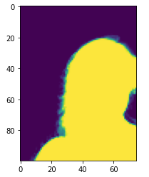
데이터 전처리
- 데이터 범위 확인
print(train_images.max(), train_images.min())
print(test_images.max(), test_images.min())- mattes의 shape을 (배치, 700, 75, 1)로 변경(흑백)
from skimage import color
train_mattes = np.array([color.rgb2gray(img).reshape((100, 75, 1)) for img in train_mattes])
test_mattes = np.array([color.rgb2gray(img).reshape((100, 75, 1)) for img in test_mattes])
train_mattes.shape, test_mattes.shape
((1700, 100, 75, 1), (300, 100, 75, 1))
데이터 시각화
- 이미지 5장 연속으로 확인
plt.imshow(train_images[:5].transpose([1, 0, 2, 3]).reshape((100,-1,3)))
plt.show()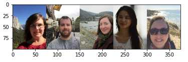
plt.imshow(train_mattes[:5].transpose([1, 0, 2, 3]).reshape((100,-1)), cmap = 'gray')
plt.show()
AutoEncoder 모델링
from keras.layers import Dense, Input, Conv2D, UpSampling2D, Flatten, Reshape
from keras.models import Model

def ae_like():
  inputs = Input((100, 75, 3))
  x = Conv2D(32, 3, 2, activation = 'relu', padding = 'same')(inputs)
  x = Conv2D(64, 3, 2, activation = 'relu', padding = 'same')(x)
  x = Conv2D(128, 3, 2, activation = 'relu', padding = 'same')(x)
  x = Flatten()(x)
  latent = Dense(10)(x)

  x = Dense((13 * 10 * 128))(latent)
  x = Reshape((13, 10, 128))(x)

  x = UpSampling2D(size = (2,2))(x)
  x = Conv2D(128, (2,2), (1,1), activation='relu', padding = 'valid')(x)

  x = UpSampling2D(size = (2,2))(x)
  x = Conv2D(64, (1,1), (1,1), activation='relu', padding = 'valid')(x)

  x = UpSampling2D(size = (2,2))(x)
  x = Conv2D(32, (1,2), (1,1), activation='relu', padding = 'valid')(x)

  x = Conv2D(1, (1,1), (1,1), activation='sigmoid')(x)

  model = Model(inputs, x)
  return model

model = ae_like()
model.summary()
오토인코더는 단순히 입력을 출력으로 복사하는 간단한 신경망으로 데이터의 차원을 축소한 후 원본 입력을 복원할 수 있도록 학습시키는 등 다양한 오토인코더가 존재한다.
- 모델에 로스, 옵티마이저, 메트릭 설정 후 학습
model.compile(loss = 'mse', optimizer='adam', metrics = ['accuracy'])
hist = model.fit(train_images, train_mattes, validation_data=(test_images, test_mattes), epochs = 25, verbose = 1)

plt.plot(hist.history['accuracy'], label = 'accuracy')
plt.plot(hist.history['loss'], label = 'loss')
plt.plot(hist.history['val_accuracy'], label = 'val_accuracy')
plt.plot(hist.history['val_loss'], label = 'val_loss')
plt.legend(loc = 'right')
plt.show()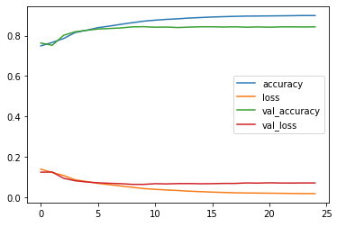
결과 확인
res = model.predict(test_images[0:1])
plt.imshow(np.concatenate([res[0], test_mattes[0]]).reshape((2, -1, 75, 1)).transpose([1, 0, 2, 3]).reshape((100, -1)), cmap = 'gray')
plt.show()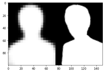
- res값을 0.5를 기준으로 0과 1로 이원화 후 다시 출력
plt.imshow(np.concatenate([(res[0]>0.5).astype(np.float64), test_mattes[0]]).reshape((2,-1,75,1)).transpose([1,0,2,3]).reshape((100,-1)), cmap = 'gray')
plt.show()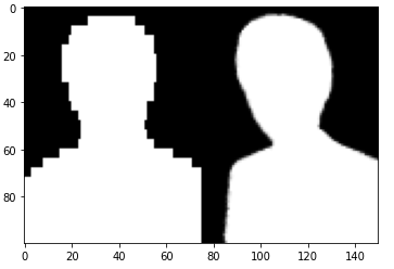
- test_images와 res를 곱한뒤 확인
plt.figure(figsize = (8,8))
plt.subplot(121)
plt.imshow(test_images[0] * test_mattes[0].reshape((100,75,1)))

plt.subplot(122)
plt.imshow(test_images[0] * model.predict(test_images[0:1]).reshape((100,75,1)))

plt.show()
성능이 그다지 정확해 보이지는 않는다.
U-net 모델링

u-net이란 Biomedical 분야에서 이미지 분할(Image Segmentation)을 목적으로 제안된 End-to-End 방식의 Fully-Convolutional Network 기반 모델을 말한다.
#간단한 U-net모델 생성
from keras.layers import Dense, Input, Conv2D, Conv2DTranspose, Flatten, Reshape, concatenate
from keras.models import Model
from keras.layers import BatchNormalization, Dropout, Activation, MaxPool2D

def conv2d_block(x, channel):
  x = Conv2D(channel, 3, padding = 'same')(x)
                      #커널
  x = BatchNormalization()(x)
  x = Activation('relu')(x)

  x = Conv2D(channel, 3, padding = 'same')(x)
  x = BatchNormalization()(x)
  x = Activation('relu')(x)
  return x

def unet_like():
  inputs = Input((100, 75, 3))

  c1 = conv2d_block(inputs, 16)
  p1 = MaxPool2D((2,2))(c1)
  p1 = Dropout(0.1)(p1)

  c2 = conv2d_block(p1, 32)
  p2 = MaxPool2D((2,2))(c2)
  p2 = Dropout(0.1)(p2)

  c3 = conv2d_block(p2, 64)
  p3 = MaxPool2D((2,2))(c3)
  p3 = Dropout(0.1)(p3)

  c4 = conv2d_block(p3, 128)
  p4 = MaxPool2D((2,2))(c4)
  p4 = Dropout(0.1)(p4)

  c5 = conv2d_block(p4, 256)

  u6 = Conv2DTranspose(128, 2, 2, output_padding=(0,1))(c5)
  u6 = concatenate([u6, c4]) # 사이즈 128
  u6 = Dropout(0.1)(u6)
  c6 = conv2d_block(u6, 128)

  u7 = Conv2DTranspose(64, 2, 2, output_padding=(1,0))(c6)
  u7 = concatenate([u7, c3])
  u7 = Dropout(0.1)(u7)
  c7 = conv2d_block(u7, 64)

  u8 = Conv2DTranspose(32, 2, 2, output_padding=(0,1))(c7)
  u8 = concatenate([u8, c2])
  u8 = Dropout(0.1)(u8)
  c8 = conv2d_block(u8, 32)

  u9 = Conv2DTranspose(16, 2, 2, output_padding=(0,1))(c8)
  u9 = concatenate([u9, c1])
  u9 = Dropout(0.1)(u9)
  c9 = conv2d_block(u9, 16)

  outputs = Conv2D(1, (1,1), activation = 'sigmoid')(c9)

  model = Model(inputs, outputs)
  return model

model = unet_like()
model.summary()- 마찬가지로 로스, 옵티마이저, 메트릭 설정 후 학습
model.compile(loss = 'mse', optimizer='adam', metrics = ['accuracy'])
hist = model.fit(train_images, train_mattes, validation_data=(test_images, test_mattes), epochs = 25, verbose = 1)

plt.plot(hist.history['accuracy'], label = 'accuracy')
plt.plot(hist.history['loss'], label = 'loss')
plt.plot(hist.history['val_accuracy'], label = 'val_accuracy')
plt.plot(hist.history['val_loss'], label = 'val_loss')
plt.legend(loc = 'right')
plt.show()
결과 확인
res = model.predict(test_images[0:1])
plt.imshow(np.concatenate([res[0], test_mattes[0]]).reshape((2,-1,75,1)).transpose([1,0,2,3]).reshape((100,-1)), cmap = 'gray')
plt.show()
- res값을 0.5를 기준으로 0과 1로 이원화 후 다시 출력
imgs = np.concatenate([(res>0.5).astype(np.float64).reshape((100,75,1)), test_mattes[0]]).reshape((2,-1,75,1)).transpose((1,0,2,3)).reshape((100,-1))
plt.imshow(imgs, cmap = 'gray')
plt.show() 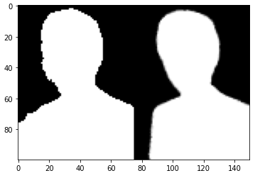
정확하지는 않지만 오토인코더보다 성능이 더 좋은것을 확인.
- test_images와 res를 곱한뒤 확인
plt.figure(figsize = (8,8))
plt.subplot(121)
plt.imshow(test_images[0] * test_mattes[0].reshape((100,75,1)))

plt.subplot(122)
plt.imshow(test_images[0] * model.predict(test_images[0:1]).reshape((100,75,1)))

plt.show()
다른 데이터도 확인
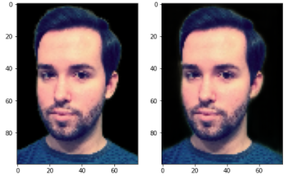
성능이 꽤 괜찮은 것 같다.
'딥러닝' 카테고리의 다른 글
| 흑백 사진을 컬러 사진으로 변경하기(U-net) (0) | 2022.03.15 |
|---|---|
| 컬러 사진을 흑백 사진으로 변경하기(U-net) (0) | 2022.03.15 |
| 화질 개선 - 손상된 이미지 화질 복구하기 (0) | 2022.03.15 |
| 인물 사진에서 성별과 표정 분류 모델(celebA) (0) | 2022.03.14 |
| Pytorch - MNIST 데이터로 MLP 모델 실습 (0) | 2022.02.05 |


