데이터 불러오기
앞서 사용한 데이터 계속 사용
- 데이터 출처 : pfcn_small
import tensorflow as tf
from tensorflow import keras
from keras.layers import Dense
from keras.models import Sequential

import pandas as pd
import numpy as np
import matplotlib.pyplot as plt
import seaborn as sns
import warnings
from IPython.display import Image

warnings.filterwarnings('ignore')
%matplotlib inline

from google.colab import drive
drive.mount('/gdrive', force_remount=True)
pfcn_small = np.load('/gdrive/My Drive/Colab Notebooks/data/pfcn_small.npz')
train_big_images = pfcn_small['train_images']
test_big_images = pfcn_small['test_images']
데이터 전처리
- 이미지의 크기를 (50, 37, 3)으로 줄인 input 데이터 생성
from skimage.transform import resize
train_small_images = np.array([resize(img, (50, 37))for img in train_big_images])
test_small_images = np.array([resize(img, (50, 37))for img in test_big_images])- 데이터 범위 확인
print(train_big_images.min(), train_big_images.max())
print(test_big_images.min(), test_big_images.max())
0.0 1.0
0.0 1.0
데이터 시각화
- 원본 데이터 확인
plt.imshow(train_big_images[:5].transpose((1,0,2,3)).reshape((100, -1, 3)))
plt.show()
- small 데이터 확인
plt.imshow(train_small_images[:5].transpose((1, 0, 2, 3)).reshape((50, -1, 3)))
plt.show()
원본보다 화질이 많이 떨어지는 것을 확인
모델링(U-net)
- small 데이터를 big으로 변경하는 모델
from keras.layers import Dense, Input, Conv2D, Conv2DTranspose, Flatten, Reshape, MaxPool2D, BatchNormalization, Dropout, Activation, concatenate
from keras.models import Model

def conv2d_block(x, channel):
  x = Conv2D(channel, 3, padding = 'same')(x)
  x = BatchNormalization()(x)
  x = Activation('relu')(x)

  x = Conv2D(channel, 3, padding = 'same')(x)
  x = BatchNormalization()(x)
  x = Activation('relu')(x)

  return x

def unet_resolution():
  inputs = Input((50, 37, 3))

  c1 = conv2d_block(inputs, 16)
  p1 = MaxPool2D(2)(c1)
  p1 = Dropout(0.1)(p1)

  c2 = conv2d_block(p1, 32)
  p2 = MaxPool2D(2)(c2)
  p2 = Dropout(0.1)(p2)

  c3 = conv2d_block(p2, 64)
  p3 = MaxPool2D(2)(c3)
  p3 = Dropout(0.1)(p3)

  c4 = conv2d_block(p3, 128)
  p4 = MaxPool2D(2)(c4)
  p4 = Dropout(0.1)(p4)

  c5 = conv2d_block(p4, 256)

  u6 = Conv2DTranspose(128, 2, 2)(c5)
  u6 = concatenate([u6, c4])
  u6 = Dropout(0.1)(u6)
  c6 = conv2d_block(u6, 128)

  u7 = Conv2DTranspose(64, 2, 2, padding = 'valid', output_padding = (0,1))(c6)
  u7 = concatenate([u7, c3])
  u7 = Dropout(0.1)(u7)
  c7 = conv2d_block(u7, 64)

  u8 = Conv2DTranspose(32, 2, 2, padding = 'valid', output_padding = (1,0))(c7)
  u8 = concatenate([u8, c2])
  u8 = Dropout(0.1)(u8)
  c8 = conv2d_block(u8, 32)

  u9 = Conv2DTranspose(16, 2, 2, padding = 'valid', output_padding = (0,1))(c8)
  u9 = concatenate([u9, c1])
  u9 = Dropout(0.1)(u9)
  c9 = conv2d_block(u9, 16)

  u10 = Conv2DTranspose(16, 2, 2, padding = 'valid', output_padding = (0,1))(c9)
  outputs = Conv2D(3, 1, activation = 'sigmoid')(u10)
  model = Model(inputs, outputs)
  return model

model = unet_resolution()
model.summary()- 모델에 로스, 옵티마이저, 메트릭 설정 후 학습
model.compile(loss='mse', optimizer='adam', metrics=['accuracy'])
hist = model.fit(train_small_images, train_big_images, validation_data=(test_small_images, test_big_images), epochs = 25, verbose=1)- 학습 진행 사항 출력
plt.plot(hist.history['accuracy'], label = 'accuracy')
plt.plot(hist.history['loss'], label = 'loss')
plt.plot(hist.history['val_accuracy'], label = 'val_accuracy')
plt.plot(hist.history['val_loss'], label = 'val_loss')
plt.legend(loc = 'right')
plt.show()
결과 확인
- test_image 1장의 결과를 res 변수에 저장
res = model.predict(test_small_images[4:5])
res.shape, test_small_images[4:5].shape
((1, 100, 75, 3), (1, 50, 37, 3))
- small 사진, 모델 결과, 원본 이미지 비교
exp = resize(test_small_images[4], (100,75))
imgs = np.concatenate([exp, res[0], test_big_images[4]],axis = 1)
plt.imshow(imgs)
완벽하진 않지만 화질이 개선된 것을 확인할 수 있다.- 여러장의 사진을 확인
res = model.predict(test_small_images[:3])
exps = np.array([resize(img, (100, 75)) for img in test_small_images[:3]])
imgs = np.concatenate([exps, res, test_big_images[:3]], axis = 2).reshape((300,-1,3))
plt.imshow(imgs)
SRCNN
- SRCNN이란?

SRCNN은 저해상도 이미지를 input으로 받아 일련의 과정을 거친 뒤, 고해상도 이미지를 output으로 출력하는 모델로 간단하게 모델링을 진행 - 학습을 위한 데이터 생성(사진의 크기는 같지만 화질이 나쁜 이미지)
train_lr_images = np.array([resize(img, (100, 75)) for img in train_small_images])
test_lr_images = np.array([resize(img, (100, 75)) for img in test_small_images])

imgs = np.concatenate([train_lr_images[0], train_big_images[0]],axis = 1)
plt.imshow(imgs)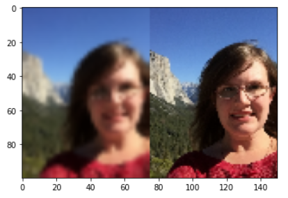
- SRCNN 모델링
from keras.layers import Average

def srcnn():
  inputs = Input((100, 75, 3))
  x = Conv2D(64, 9, activation = 'relu', padding='same')(inputs)

  x1 = Conv2D(32, 1, activation='relu', padding='same')(x)
  x2 = Conv2D(32, 3, activation='relu', padding='same')(x)
  x3 = Conv2D(32, 5, activation='relu', padding='same')(x)
  x = Average()([x1, x2, x3])

  outputs = Conv2D(3, 5, activation= 'relu', padding='same')(x)
  model = Model(inputs, outputs)
  return model

model2 = srcnn()
model2.summary()

model2.compile(loss='mse', optimizer='adam', metrics=['accuracy'])

hist2 = model2.fit(train_lr_images, train_big_images, validation_data=(test_lr_images, test_big_images), epochs = 25, verbose=1)- 학습 진행 사항 출력
plt.plot(hist2.history['accuracy'], label = 'accuracy')
plt.plot(hist2.history['loss'], label = 'loss')
plt.plot(hist2.history['val_accuracy'], label = 'val_accuracy')
plt.plot(hist2.history['val_loss'], label = 'val_loss')
plt.legend(loc = 'right')
plt.show()
- U-net모델과 결과 비교
res1 = model.predict(test_small_images[4:5])
res2 = model2.predict(test_lr_images[4:5])
imgs = np.concatenate([test_lr_images[4], res1[0], res2[0], test_big_images[4]],axis = 1)
plt.imshow(imgs)
간단한 모델이지만 srcnn의 성능이 더 뛰어나 보인다.- 여러장의 결과를 비교
res1 = model.predict(test_small_images[:3])
res2 = model2.predict(test_lr_images[:3])

imgs = np.concatenate([test_lr_images[:3], res1, res2, test_big_images[:3]], axis = 2).reshape((300,-1,3))
plt.imshow(imgs)
'딥러닝' 카테고리의 다른 글
| CNN을 이용한 Image Localization (0) | 2022.03.16 |
|---|---|
| Pre-trained 모델과 Data aungmentation(cutmix, crop, flip)을 활용한 이미지 분류 모델 (0) | 2022.03.16 |
| 흑백 사진을 컬러 사진으로 변경하기(U-net) (0) | 2022.03.15 |
| 컬러 사진을 흑백 사진으로 변경하기(U-net) (0) | 2022.03.15 |
| 사진에서 사람 영역만 구분하기(AutoEncoder, U-net) (0) | 2022.03.15 |


